|
Google Apps

Top 10 Google Sheets Tips for Productivity!

Never bothered learning how to use the advanced formulas and Google Sheet functions in spreadsheet? Fear not, learn how to create dropdown menus, checkboxes, and even org charts without having to memorize a single thing! 🤓

Watch it in action

Tip #1 - Create Filtered View

Don’t want anyone messing with your filters when collaborating on the same document? Here’s what you can do:

  1. Go to the filter icon in the menu tab > click the downward arrow
  2. Select “Create new filter view”
  3. Give your filter a name and choose what you want to filter out

ONLY you will be able to see this filtered view so this won’t affect your colleagues.

đź’ˇ
Pro Tip: If you want to share the filtered view with a colleague, send them the URL with the filtered view enabled so they are brought to it directly

Take it a step further by filtering your columns by color:

  1. Highlight the respective column > go to Format > Conditional formatting
  2. Select Format cells if “is empty” > select a color > click Done
  3. Go back to the filter icon > select All to view all your filtered areas
  4. Click on the dropdown arrow next to a filter > select Filter by color > Fill Color > choose a color

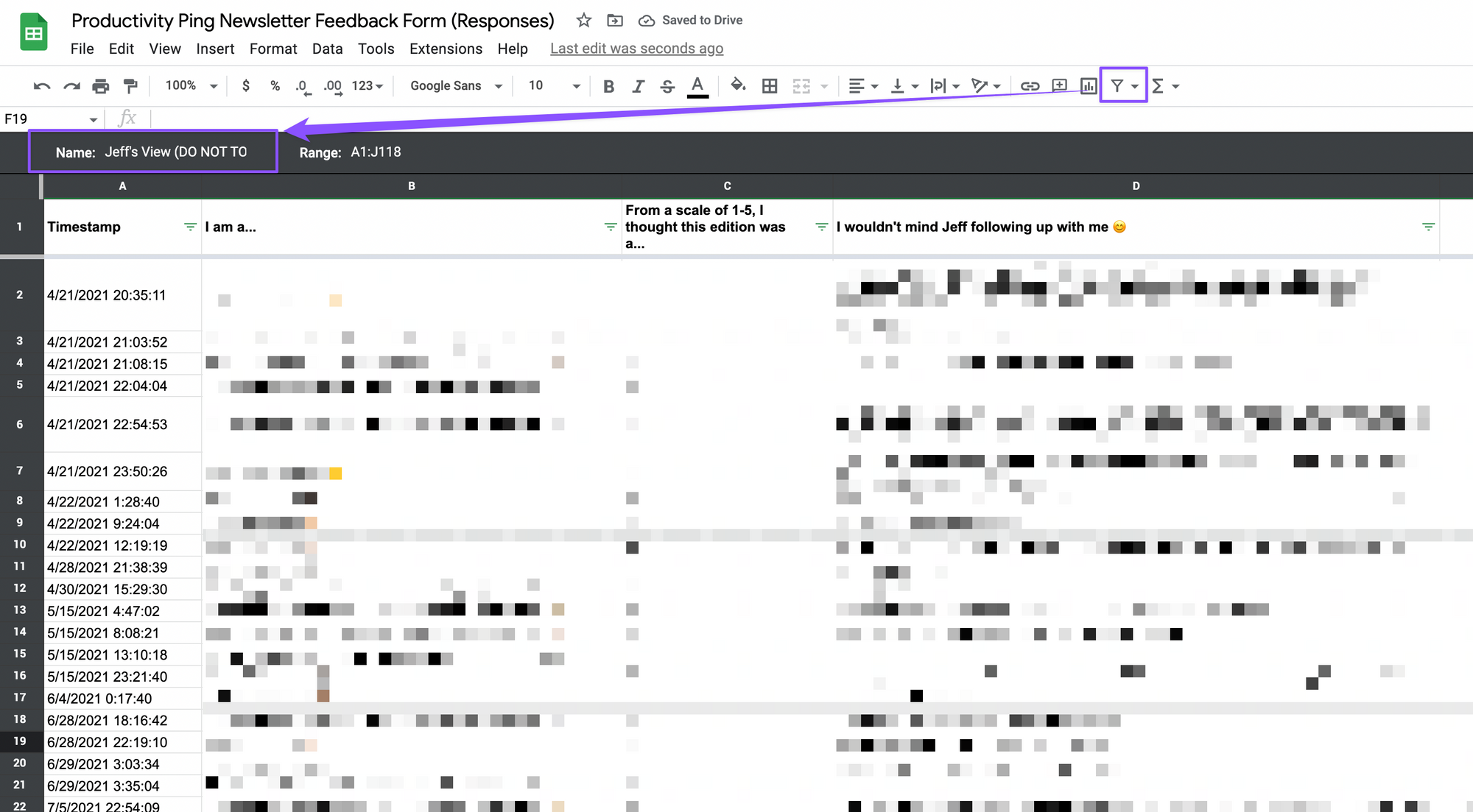
This is useful for when you need to see which tasks you have completed at a glance!

If you need someone else to input data into Sheets:

  1. Highlight the column/row you need their input for > right click > select “Get link to this range”
  2. Send the copied link to them

Once they open the link, it will take them directly to the highlighted row or column!

Tip #3 - Protect & Lock Ranges

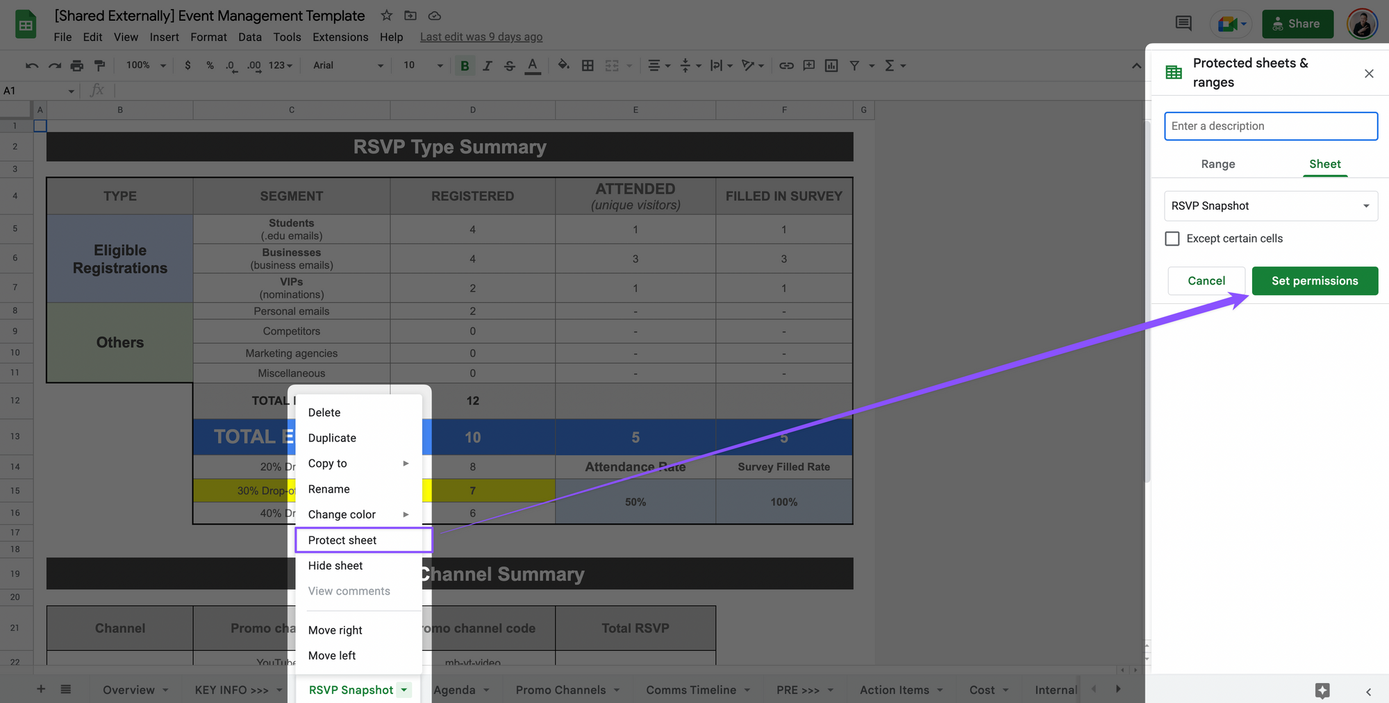
For all you control freaks, no one will mess with your files ever again.

  1. Highlight the columns/rows you want to lock > go to Data in the menu bar
  2. Select “Protected sheets and ranges”
  3. Under the Range tab > click “Set permissions” > uncheck the emails of the other collaborators > click Done

And if you came across this tip too late and the damage is already done? Read on.

Tip #4 - Show Edit History

To show the changes that have been made:

  • Right click on the cell > click “Show edit history”

This shows you every single edit that has been made…ever.

Tip #5 - Create an Org Chart in Google Sheets

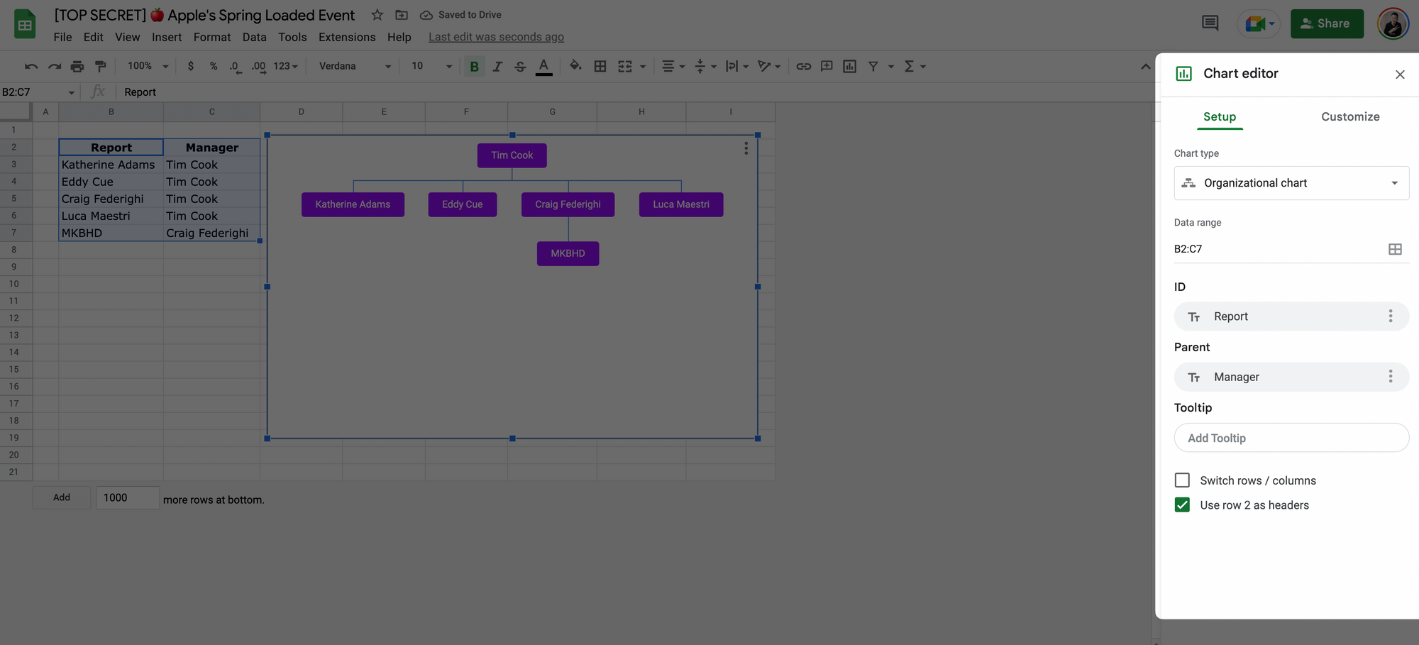
Save tons of time by creating org charts directly in Sheets instead of Powerpoint or Slides!

For example, if you already have the “Report” and “Manager” columns inputted into sheets:

  1. Highlight the two columns > go the Insert in the menu bar > select Chart
  2. Under Chart type, select the Organizational chart
  3. Under the Setup tab, enable “Use row 2 as headers”
  4. Under the Customize tab, you can choose to change the node colors
đź’ˇ
Pro Tip: Copy the chart from Sheets and paste it directly into Google Slides (make sure to “Link to spreadsheet”) for the option to update the chart automatically within the slides

Tip #6 - Turn Off Notifications

To turn off annoying notifications every time someone edits a shared document:

  • Go to notification history icon in the top right corner > click Notifications > select “Only yours”

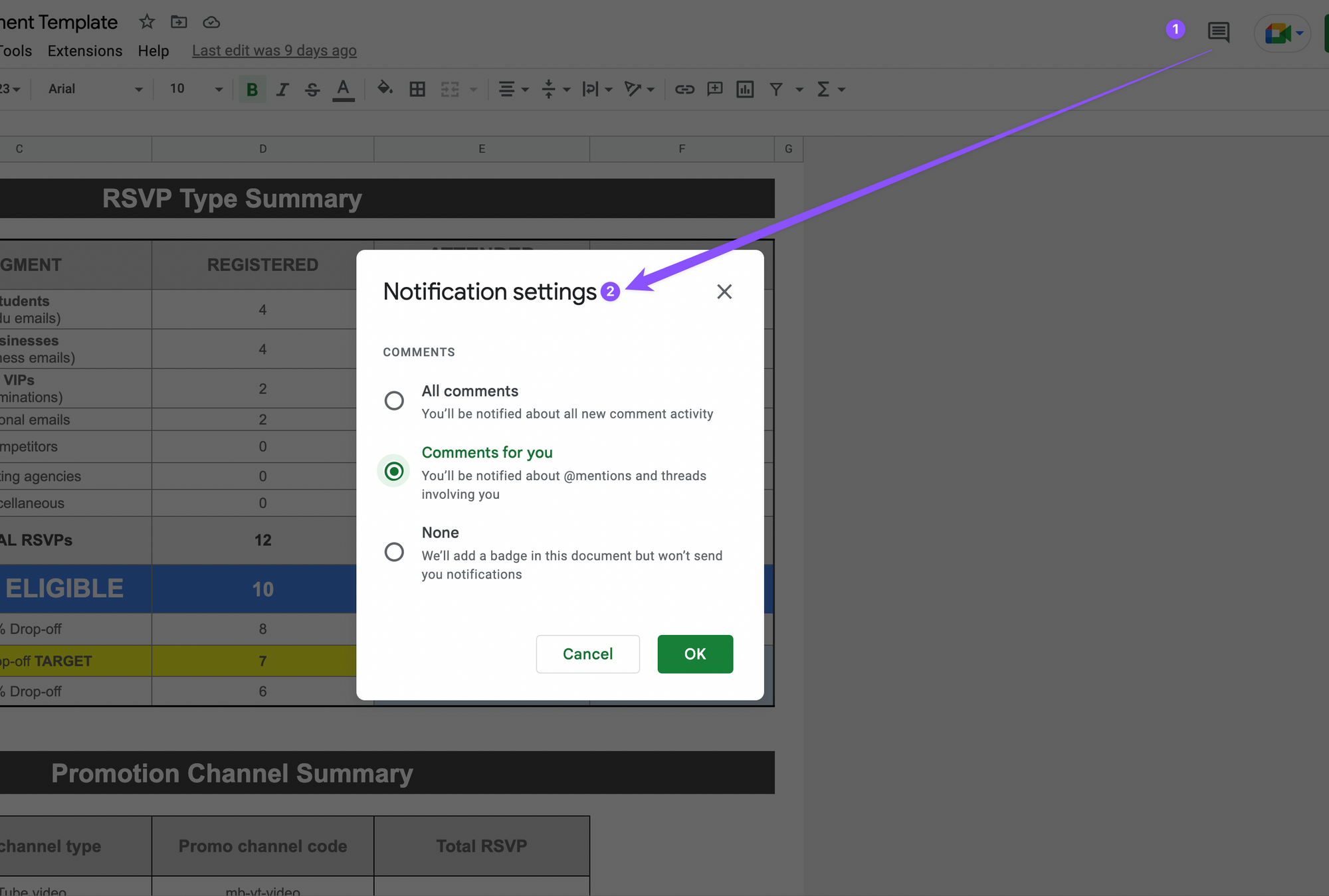
Now you’ll only be notified if someone mentions you in a comment!

Tip #7 - Top Formatting Tips

Enable alternating colors for long lists to make it easier to read:

  • Go to Format > Alternating colors > pick a color you like

Group and color-code tabs by their functions:

  • Right click on a tab > select “Change color”

Quickly enable a yes/no or checkbox option:

  • Highlight the column > go to Insert > select “Checkbox”

Tip #8 - Copy Tab Quickly

To copy an entire spreadsheet over to a new one without messing up the formatting:

  1. Right click the original tab at the bottom of the page
  2. Select “Copy to” > Existing spreadsheet
  3. Copy the URL of the spreadsheet you want to copy to > paste it and press Select

Now you should have a copy of the spreadsheet in the other document with all the formatting perfectly intact.

Tip #9 - Remove Duplicates

Instead of manually removing duplicates within your sheets:

  • Highlight the table > go to Data > Remove duplicates
  • You can choose to select the columns you want to remove duplicates for

Tip #10 - Convert Currencies

You can use the Google Finance function for currency exchange calculations.

For example, if you want to quickly see how much a product will cost from USD to HKD:

  • Within the cell, type in “=E5*GOOGLEFINANCE(“CURRENCY:USDHKD”)

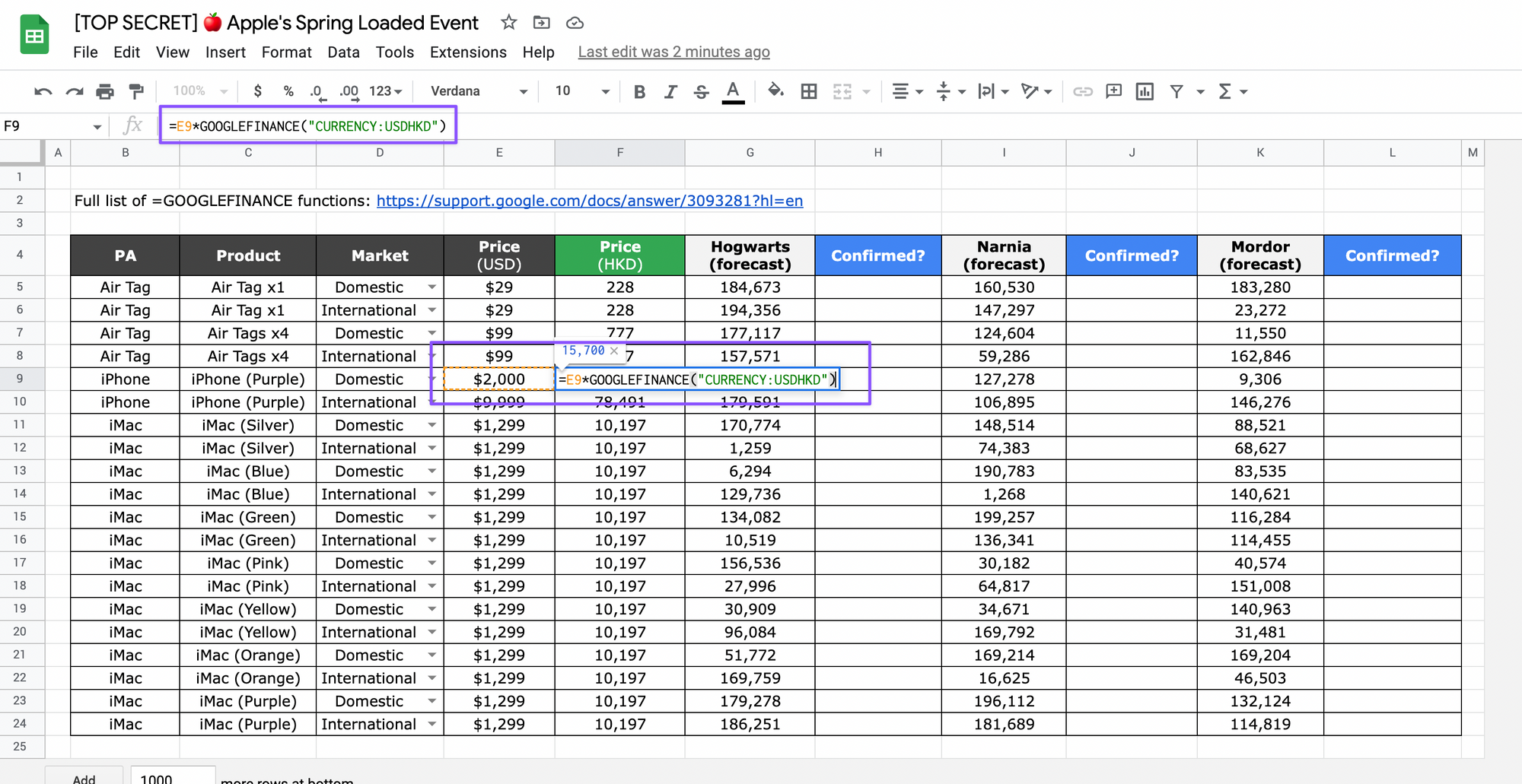
Super handy if you work with people all over the world!

For more tips on creating sexy spreadsheets…

Check out these 10 best practices for shared spreadsheets and copy a free template here!