15 Google Sheets Formulas We Should All Know!

In this post I will share some Google Sheets formulas and functions I used the most over the past 7 years as a working professional.

Watch it in action

DETECTLANGUAGE

You can use this DETECTLANGUAGE formula to identify the language code, then use the GOOGLETRANSLATE formula to find out that Jeff is simply the sweetest and that he appreciates you all very very much 😁.

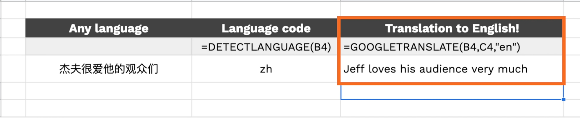
I’ll admit this formula is definitely not necessary for working professionals to know but you gotta admit it’s pretty freaking cool!

VLOOKUP MISTAKES

True vs False

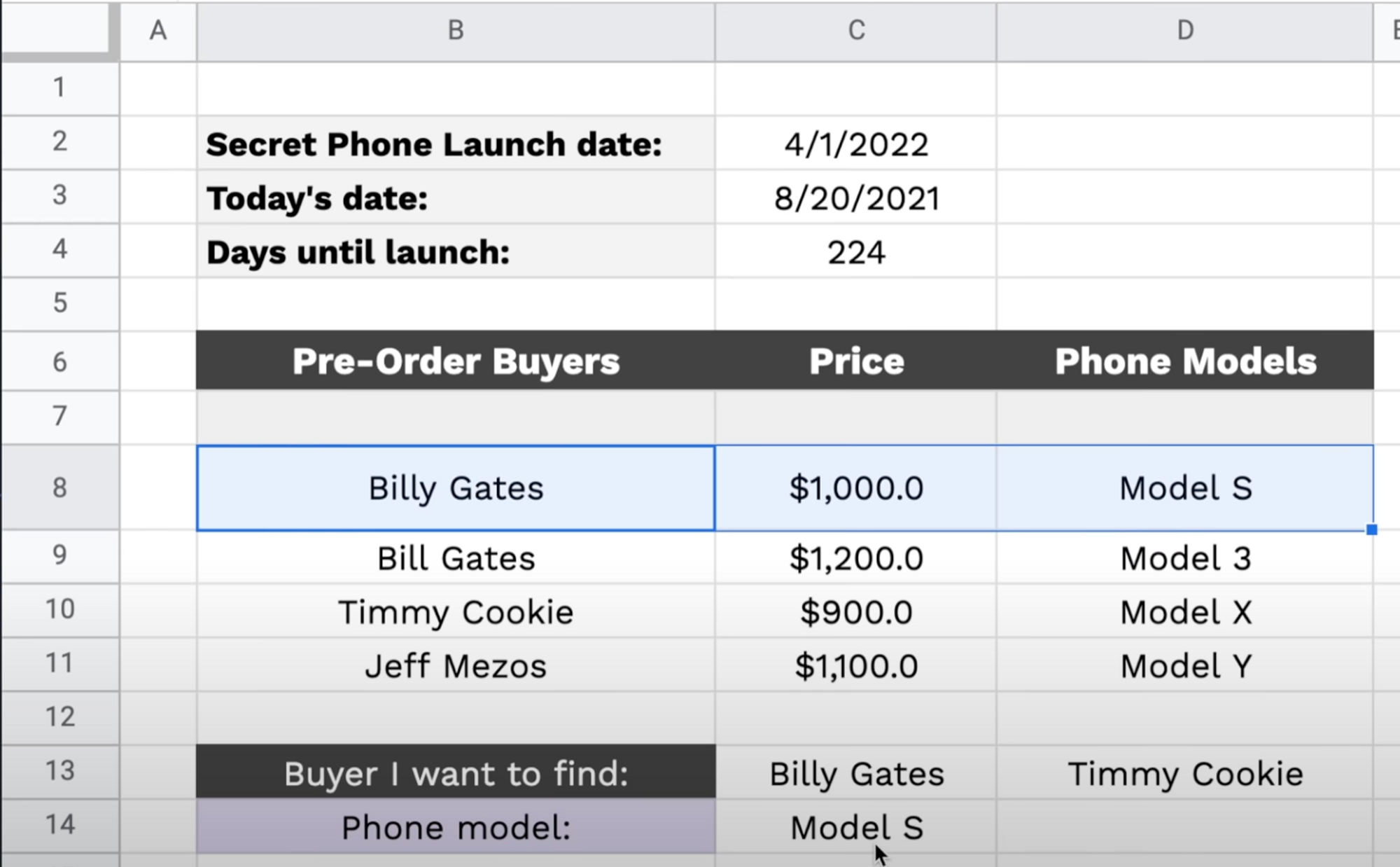
A lot of people type in “TRUE” or “1” in the VLOOKUP formula. This basically means you’re telling Google Sheets or Excel to find the closest match, but that may sometimes lead to errors.

For example, I want to find Billy Gates but because I used True, it returned the phone model that Bill Gates bought. If I simply change this to FALSE or 0, telling sheets to find the exact match, the correct phone model will be shown.

• My formula: VLOOKUP(C13,B8:D11,TRUE)

Wildcard Asterisk

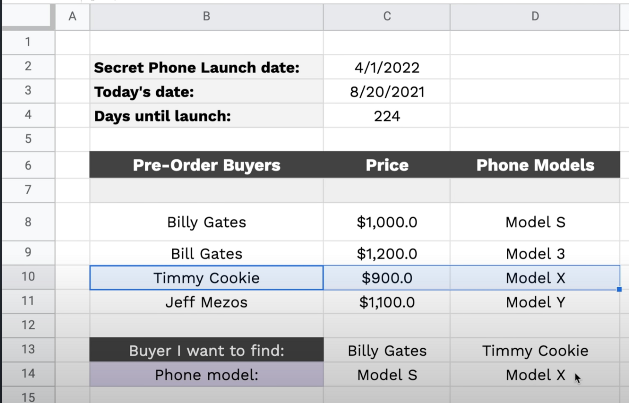
It can be very handy to use the wildcard asterisk character with the VLOOKUP formula. If you know someone’s name starts with Ti, you can simply input “Ti*” and find the corresponding output.

• My formula: =VLOOKUP(”Ti*”,B8:D11,3,FALSE)

TODAY()

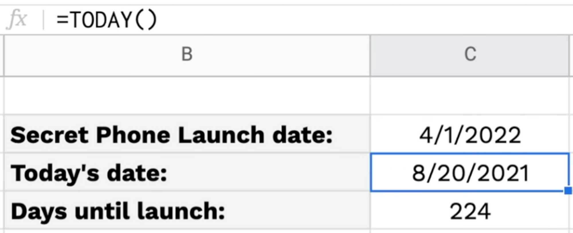
I have a “Days until launch” field whereby I subtract today’s date from the launch date. The launch date obviously does not change, but if I use the =TODAY() formula, today’s date changes everyday and “days until launch” also updates accordingly. A handy little trick that I use all the time at work.

IMPORTRANGE

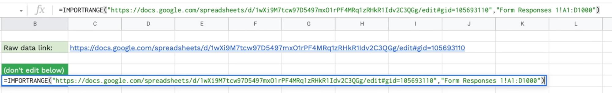
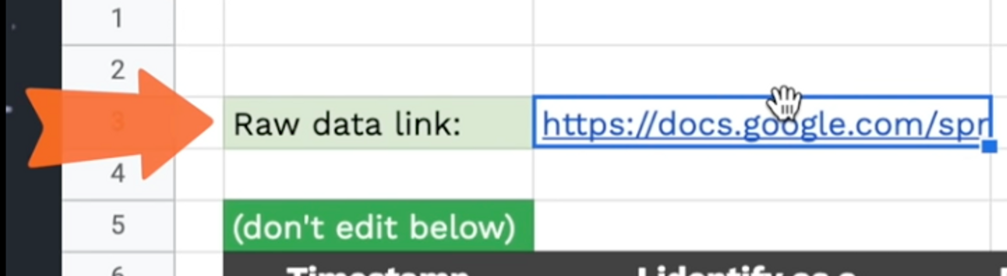
For those of you who don’t know what this is, you’re simply making an exact copy of a tab from a separate Google Sheets file, or from a tab within the same file, and the beauty of this is that when the original updates, the import range version updates as well.

• For example I have a bi-weekly productivity newsletter and I always ask for feedback via Google Forms. That Google form outputs the data in Google Sheets in real time and I could import this into a separate tab by using this formula.

If you see an error, you have to allow the connection to give access but after you do that, you should be able to see the exact same data from the other spreadsheet.

• You do this because you might want to change the formatting of the data, or analyze the data by making calculations, but you don’t want to mess with and potentially mess up the raw data.

COUNTIF

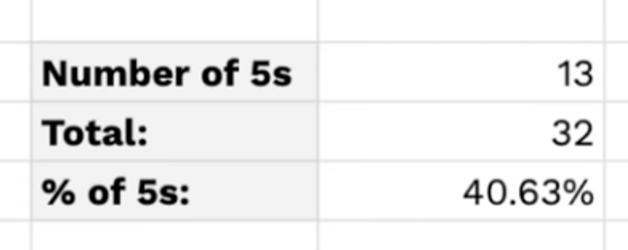
If I wanted to find the number of people who gave me 5 out of 5, I use the “COUNTIF” formula, and I want to find 5, there are 13 people who gave me 5.

• My formula: =COUNTIF(D7:D38,5)

COUNTA

If I want to know how many people are in total, I use the =COUNTA formula, and I can highlight any of the columns since it’s just calculating the number of responses total, so there are 32 responses so far.

If I wanted to find the percentage of 5s, just divide 13 and 32 and 40,6% of people gave me 5.

• My formula: =H2/H3

SPLIT

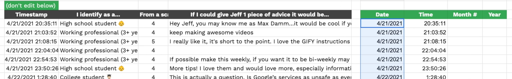
If I wanted to separate out the date and the time in the timestamp column, I can use the SPLIT formula.

For SPLIT you tell Google Sheets the cell you want to split, and the delimiter you want to split by, the most common “delimiter” is just a space. But you can always split text separated by commas for example.

I have the date and time in 2 separate columns, if I highlight the entire column, and press CMD D, or CTRL D on Windows, it will apply the formula to all the rows.

• My formula: =SPLIT(B7,” “)

ISEMAIL and SUBSTITUTE

Let’s say you receive some data from a colleague who, shall we say, isn’t the most detail oriented 🙄, and you want to double check the data before doing anything else.

ISEMAIL

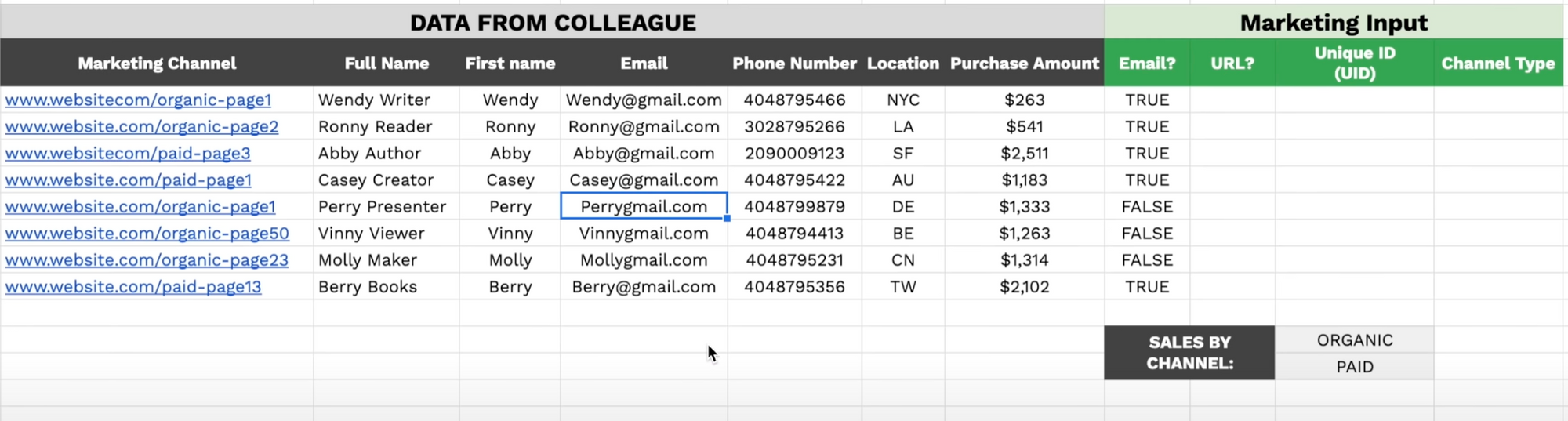
Use the ISEMAIL formula to check whether this is in fact a correctly-formatted email address.

• You simply input =ISEMAIL(cell) press enter, drag down, and you see 3 are false. It’s because there is no @ symbol between the name and the gmail domain.

SUBSTITUTE

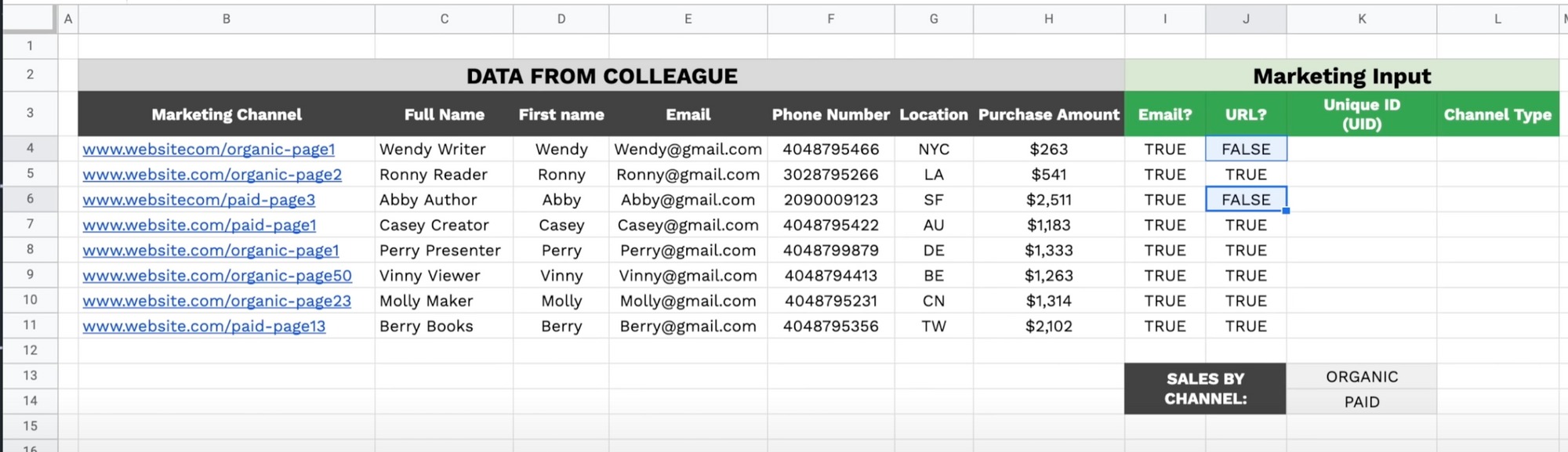
To quickly fix that, you can use the substitute formula. Press =SUBSTITUTE, select the one with the mistake up top, you want to replace “gmail.com” with “@gmail.com” and drag down. Copy and paste without formatting, and this should update to all TRUE.

• My formula: =SUBSTITUTE(E8,"gmail.com","@gmail.com")

ISURL

You can use the ISURL formula to check whether the marketing channel column does indeed contain URLs. =ISURL(cell), press enter, drag down. These 2 are false, and you’ll see that cells B6 and B4 are missing the period before “com” so similarly you can use the substitute formula to correct that.

ARRAYFORMULA

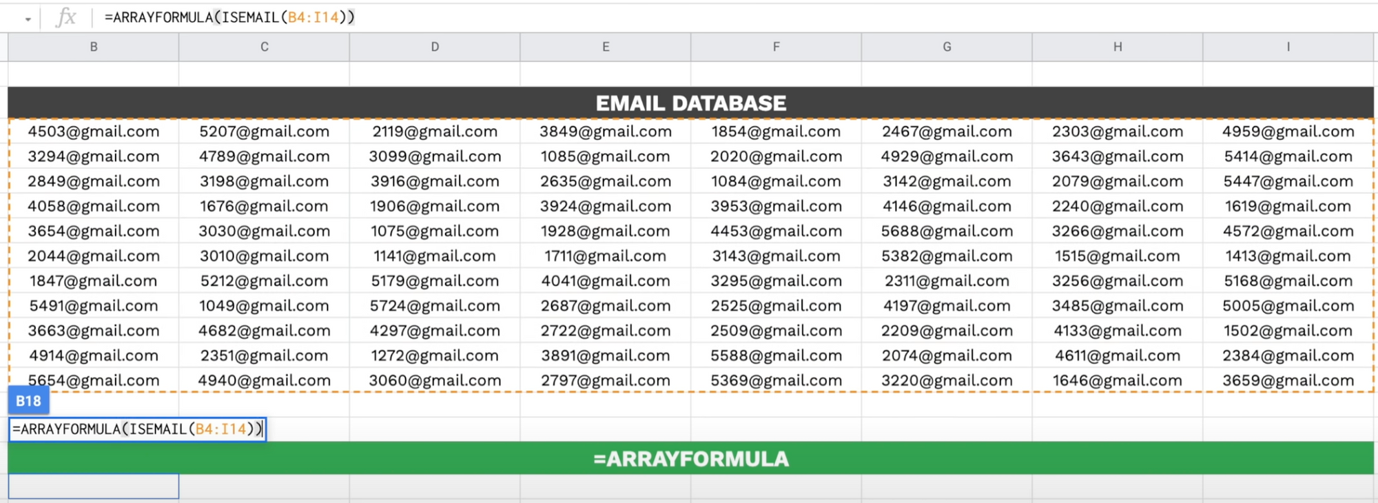
What if you’re working with a LOT of data, there are 88 emails here, and you want to check them all at once.

You can use ARRAYFORMULA and include ISEMAIL in there, and you would highlight the entire range you want to check instead of just 1 cell, and this will automatically populate all the corresponding columns and rows without you dragging the formula across and down and whatnot.

And of course ARRAYFORMULA works with almost all other formulas as well.

CONCATENATE and &

CONCATENATE

Usually you give clients a UID or Unique ID for them to use to login or identify themselves.

A very easy way to assign UIDs in bulk is to use the “CONCATENATE” formula that combines values from different cells together.

If I wanted to use their location and phone numbers to come up with a UID, I can CONCATENATE() location, and their phone number. But this is obviously not very privacy-friendly.

So you should take this a step further, use the RIGHT() formula to grab the last 4 digits of their phone number and generate an ID that is both unique and protects their identity.

• My formula: =CONCATENATE(G4,RIGHT(F4,4))

&

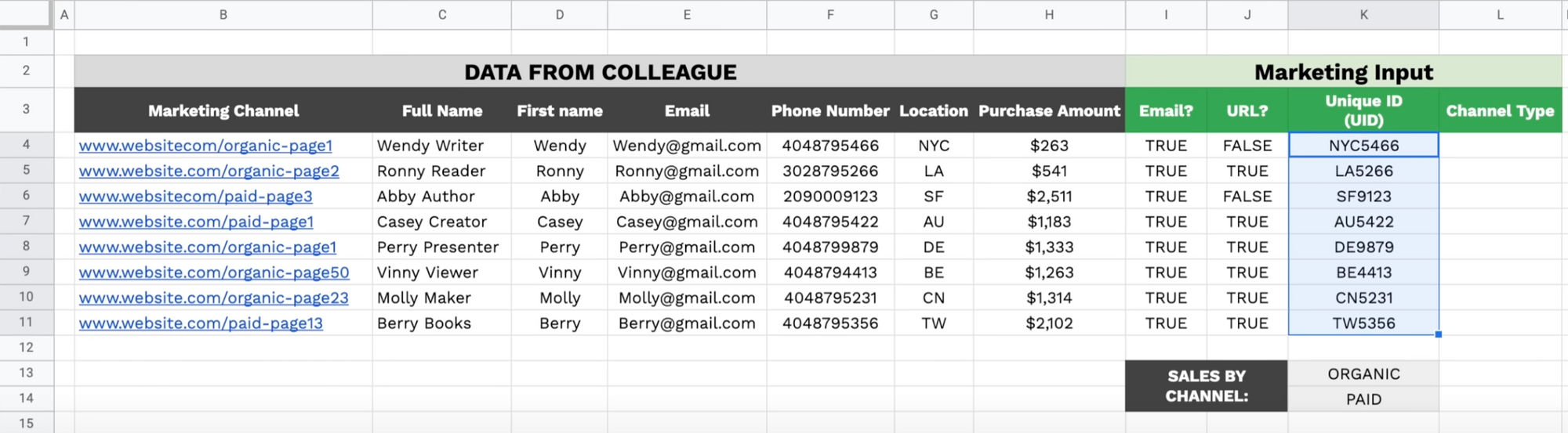
Similarly you can use the “AND” sign to achieve the same thing. I first use the LEFT formula to grab the first 3 characters of their first name, use & in between, and use the RIGHT formula to grab the last 4 digits of their phone number, and this works just as well.

• My formula: =LEFT(D4,2)&RIGHT(F4,4)

IF and SEARCH

SEARCH

Looking at the marketing channels there is organic traffic and paid traffic.

If I wanted to identify all the organic ones, I can start with =SEARCH(“organic”,cell) and if it finds the word organic, it returns 1.

IF

Then I can use the IF formula on top of it to return the word “organic” instead of the meaningless number 1.

If I drag this down, you’ll see that for non-organic traffic channels, there is an error, this is to be expected.

• My formula: =IF(SEARCH(”organic”,B6),”ORGANIC”,” “)

IFERROR

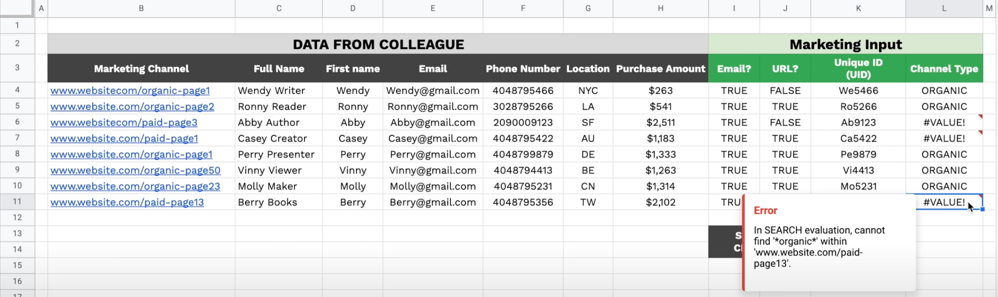
The IFERROR formula on top of the IF and SEARCH functions to return the word “PAID” if it doesn’t find the “organic” word in the initial cell. While this 3 formula combination may look a bit scary at first, the key is to start with the inside formula, and work your way out.

• My formula: =IFERROR(IF(SEARCH(”organic”,B6),”ORGANIC”,” “),”PAID”)

SUMIF

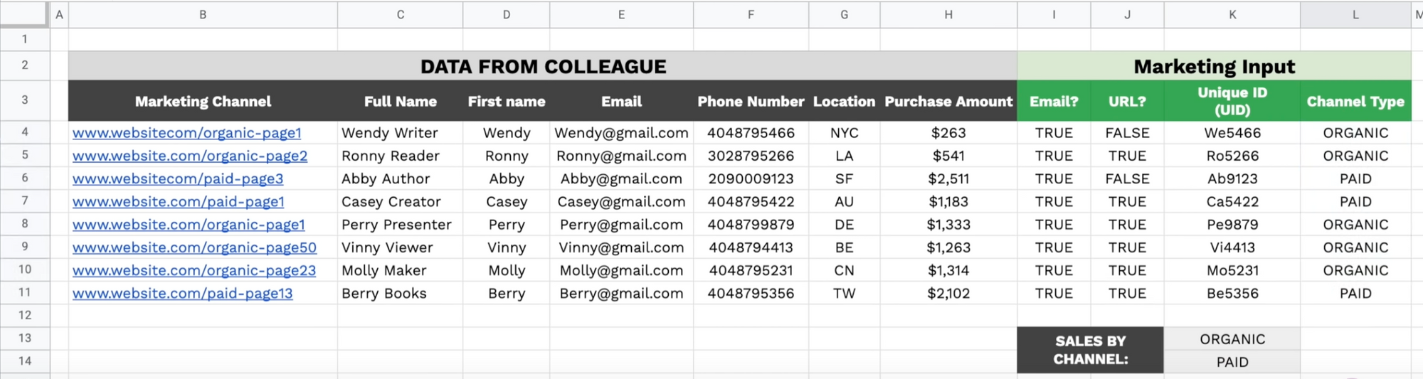
Now we’ve identified the PAID and ORGANIC channels, I want to know how much they’re contributing to sales.

I can use the SUMIF function, and first highlight the range I want to analyze, which is the channel type column, FN+F4 to lock the range in place, the criteria is the word “ORGANIC”, and the range I want to sum up is the sales numbers, FN+F4 to lock in place again.

• My formula: =SUMIF($L$4:$L$11,K13,$H$4:$H$11)

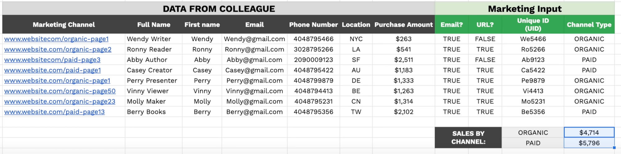
For the PAID channels, I simply paste this formula down by pressing CMD+D, and because I had already locked the ranges I know the referenced cells will not move, and I can just change the word from ORGANIC to PAID.

To get a quick sense check, these two added up is 10,000, and if I sum all this up, it’s also 10,000 so no issues there.

I want to quickly point out that yes I could have done that manually using the SUM formula or the “+” addition sign, but that’s prone to human error, especially since you’re probably working with a lot more data in real life.

• By using formulas like SUMIF correctly, it is physically impossible for you to make an error in those types of calculations.

TRIM, UPPER, LOWER and PROPER

This consists of the 4 most common formatting functions I use when I receive raw data. There are times where you need to do this before inputting the data in a database.

TRIM

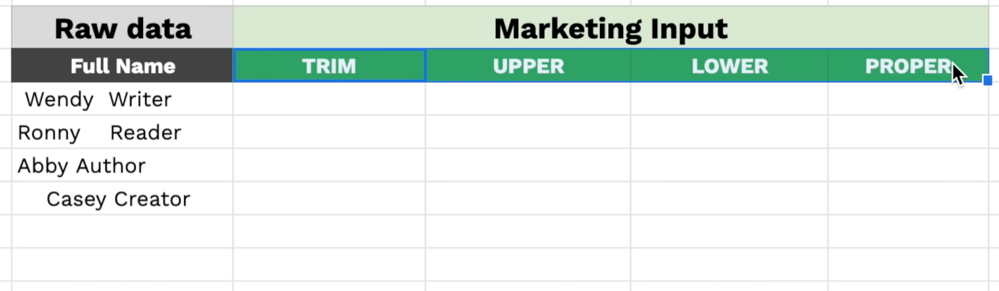
For example there are just random spaces sometimes and to get rid of them you use the TRIM formula.

• My formula: TRIM(B4)

UPPER

If I wanted to convert all the letters to uppercase, I would use the UPPER formula.

• My formula: UPPER(C4)

LOWER

If I wanted to convert all the letters to lowercase, I would use the LOWER formula.

• My formula: LOWER(D4)

PROPER

For capitalizing the first letter of each word, use the PROPER formula.

• My formula: PROPER(E4)

For more tips and tricks...

Check out my Top 10 Google Sheets Tips for Productive Professionals video!